Combined X-ray/neutron refinement – PbSO₄

A video version of this tutorial is available at https://anl.box.com/v/Combinedrefinement

Exercise files are found here

In this training exercise you will refine the structure of lead sulphate using both constant wavelength X-ray and neutron data. The problem here is that the two experiments were done at different temperatures (X-ray at room temperature & neutron at low temperature) so the patterns don’t correspond to the same lattice parameters. The structure is orthorhombic with five different atomic sites. The exercise will finish with the generation of the two Fourier maps and you can then see the effects the different neutron scattering lengths and x-ray scattering factors have on the maps. The neutron data was taken on the D1a powder diffractometer at the ILL, Grenoble, France using 1.909Å wavelength neutrons, while the x-ray data was taken on a standard laboratory Bragg-Brentano diffractometer with Cu Ka radiation.

We recommend that you do the two exercises Laboratory X-ray Powder Data and Neutron CW Powder Data Rietveld refinements.

If you have not done so already, start GSAS-II.

Step 1: Read in the data files

1. Use the Import/Powder Data/from GSAS powder data file menu item to read the first data file into GSAS-II. This read option is set to read any of the powder data formats defined for GSAS (angles in centidegrees). Other submenu items will read the cif format or the xye format (angles in degrees) used by Topas, etc. Change the file directory to CWCombined/data to find the file; you will need to change the file type to All files (*.*) to find the desired file.

2. Select the PBSO4.CWN data file in the file dialog and press Open. There will be a Dialog box asking Is this the file you want? Press Yes button to proceed. NB: don’t be tempted to also read in the PBSO4.XRA file at the same time; GSAS-II will apply the same instrument parameter file (next step) to both!

3. Select the inst_d1a.prm instrument parameter file in the second dialog and press Open. The plot will show the neutron powder data.

4. Again use Import/Powder Data/from GSAS powder data file menu item to read the second data file into GSAS-II; ; you will need to change the file type to All files (*.*) to find the desired file.

5. Select the PBSO4.XRA data file in the file dialog and press Open. There will be a Dialog box asking Is this the file you want? Press Yes button to proceed.

6. Select the INST_XRY.PRM instrument parameter file in the second dialog and press Open. On the plot press the m key; the plot will show both data sets; the x-ray one as blue ‘+’ marks and the neutron one as a blue curve.

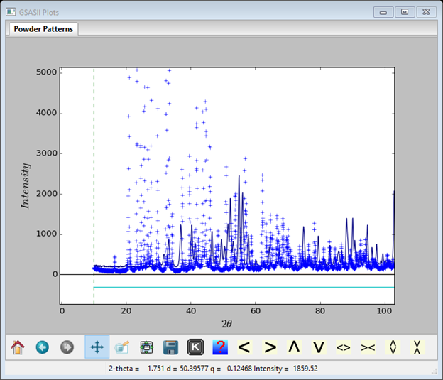
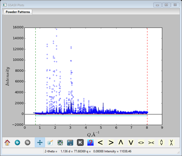
If you set the focus on the plot (press a mouse button with the cursor in the plot frame) and then press ‘q’, the plot will be redrawn with q(=2p/d) as the x-axis putting both data sets on the same scale for easier comparison.

The GSAS-II data tree now has two sets of PWDR entries; they can be distinguished by their different data set names. I’ve expanded the window so the entire data tree is shown here.

Step 2. Enter the phase information for PbSO₄

Lead sulphate has the same structure as BaSO₄; we will start with the crystallographic information given in Wycoff (“Crystal Structures Vol 3, p 46). The space group is P n m a (don’t forget the spaces between the axial fields) with a = 8.480, b = 5.398 and c = 6.958. The coordinates given by Wycoff are

Type	X	Y	Z
Pb	0.1882	0.25	0.167
S	0.063	0.25	0.686
O	-0.095	0.25	0.600
O	0.181	0.25	0.543
O	0.085	0.026	0.806

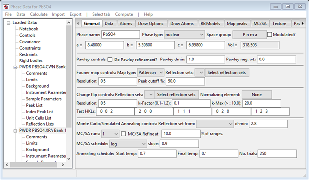
Begin by selecting Data/Add new phase in the GSAS-II data tree menu, use PbSO4 for the phase name and then fill in the space group and lattice parameters in the General tab of the Phase data for PbSO4 window. When done, you should have

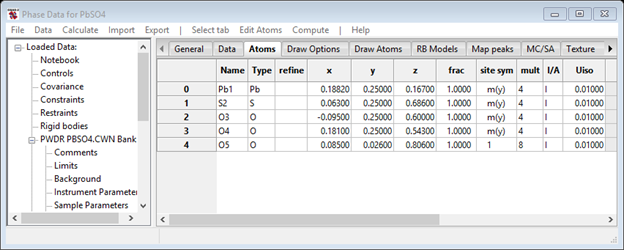
Next select the Atoms tab, select Edit Atoms/Append atom 5 times to fill in sufficient blank atoms for this structure. Then fill in the atom Type and xyz positions. When done, you should have

Step 3. Add data to the phase

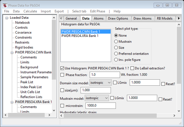
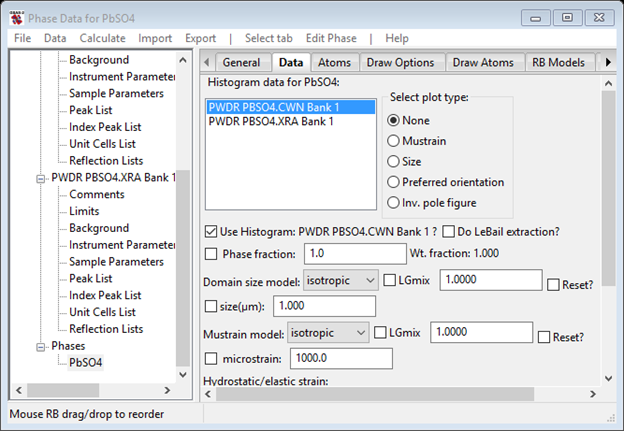
Next you have to select the powder patterns to be used for the PbSO₄ phase. To start select the Data tab of the Phase data for PbSO4 window. Then select the Edit Phase/Add powder histograms menu item; select SetAll to include both patterns and press OK. The Phase data for PBSO4 window will list both patterns

Step 4. 1^st Rietveld refinement

Now do a preliminary Rietveld refinement; GSAS-II will first ask for a project file name. We assume NXPbSO4.gpx is used (don’t put in the extension). The refinement will finish with Rwp~18% for the neutron data and Rwp~41% for the X-ray pattern. Now look closely at the fit. The plot should be in Q and with just one pattern selected (use ‘q’ and ‘m’ options on the plot to get there). Although the fit is poor, the calculated peaks appear to be close to the right positions in the x-ray pattern

but are shifted to lower Q in the neutron pattern.

This is the result of thermal expansion of PbSO₄ and the lower temperature used for the neutron data collection.

Step 5. Select some parameters and 2^nd Rietveld refinement

To improve the refinement you should first select the checkbox to Refine unit cell in the General tab of the Phase data for PbSO4 window and then select Calculate/Refine in the GSAS-II data tree window. The x-ray Rwp will improve (~38%) but the neutron Rwp will be a bit worse (~20%) as the least squares seeks a global minimum.

Step 6. Allow for thermal expansion and 3^rd Rietveld refinement

In GSAS-II there are explicit parameters for thermal “strain”; find them in the Data tab in the Phase data for PbSO4 window. Select the PWDR PBSO4.CWN entry for the neutron data. I’ve expanded the window slightly to see everything

Select the three parameters (D11, D22 and D33) under Hydrostatic/Elastic strain for refinement and do another Rietveld refinement. There is immediate improvement for both data sets; the neutron Rwp~15% and the x-ray Rwp~31%. Moreover, the peaks are in the right places for both data sets, although the shapes aren’t right. We will deal with them next.

Step 7. Crystallite size and mustrain selection and 4^th Rietveld refinement

The peak shapes are affected by sample broadening; the relevant parameters are found in the Data tab of Phase data for PbSO4 window. There is a set for each powder pattern. However, the neutron data is of much lower resolution than the x-ray data and is thus less sensitive to sample broadening effects. Select Cryst. size(mm) and microstrain only for the x-ray data (2 parameters) and then do another Rietveld refinement. The x-ray fit is significantly improved (Rwp~26%) while the neutron fit is unchanged (Rwp~15%). Examine the two plots in detail; the neutron plot shows mostly differences in peak intensity and the x-ray data shows differences in peak positions.

Step 8. Structure and x-ray sample displacement and 5^th Rietveld refinement

The peak intensity differences in the neutron case are more apparent than in the x-ray case because all atoms contribute about equally to the neutron scattering, while the Pb atom dominates the x-ray pattern. On the other hand, the sample position in a Bragg-Brentano diffractometer is almost never properly located tangent to the focusing circle and the sample position for something inside a cryostat on a neutron diffractometer isn’t very well known either So we’ll refine these things next.

1. Select the PWDR PBSO4.XRA BANK 1 item in the GSAS-II data tree and select Sample Parameters. Check Sample displacement for refinement and make sure Bragg-Brentano is the Diffractometer type.

2. Select the PWDR PbSO4.CWN Bank 1 item and select Sample Parameters. Make sure Diffractometer type is Debye-Scherrer then change Goniometer radius to 650 mm and check both Sample X & Sample Y displ. parameters for refinement.

3. Select Phases/PbSO4 in the GSAS-II data tree and select the Atoms tab. Double click the refine column heading. Select X and U for refinement and press OK.

4. Do the Rietveld refinement. The fit improves on both patterns; Rwp=7.05% for the neutron data and Rwp=12.09% for the x-ray data.

If you look at Sample Parameters for the neutron pattern, you’ll see that the sample position is about 2mm off in the X-direction & 1mm off in the Y-direction. Compare this to the X-ray data where the sample is displaced ~75μm. Both had a substantial effect on the fit.

Step 9. Instrument parameters and 6^th Rietveld refinement

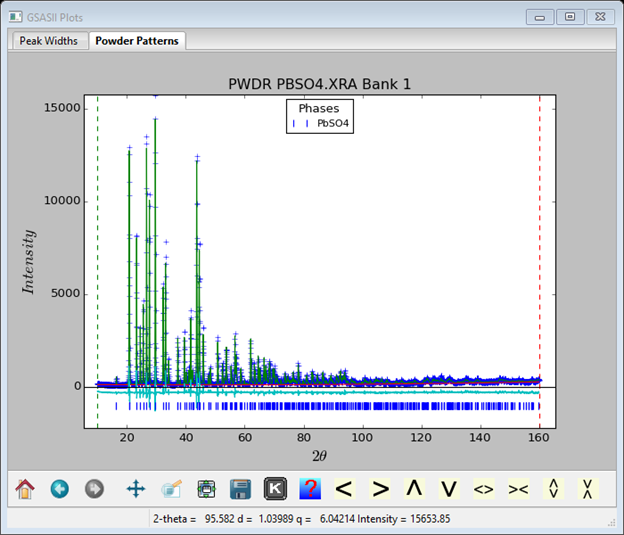
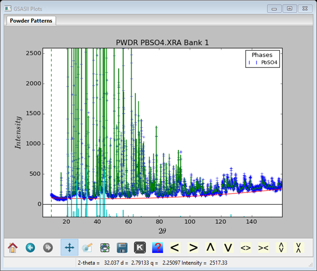
Finally (perhaps), we can do the refinement of the U, V and & W Gaussian profile parameters for both data sets. These are found in the Instrument Parameters item under each PWDR entry in the GSAS-II data tree. Don’t refine the x-ray or neutron Zero, that isn’t usually the problem if the instrument is reasonably well cared for (zero calibration makes it 0.001° or better); we’ve already dealt with peak offset issues by refining sample positions Additional changes to consider are to move the lower limit on the x-ray and neutron data to just below the 1^st peak, set the upper limit to the gap just below the end of the neutron pattern. With this the final Rwp=4.53% for the neutron data and Rwp=10.99% for the x-ray data. The x-ray plot is

I adjusted the plot with the Pan button and repositioned the reflection tick marks; they can be dragged anywhere with the mouse. The neutron pattern looks like

Again I repositioned the plot and the reflection tick marks. The NXPbSO4.lst file contains the complete refinement results (some lines have been trimmed).

Refinement results:

--------------------------------------------------------------------------------------

Number of function calls: 9 No. of observations: 8870 No. of parameters: 41

User rejected: 0 Sp. gp. extinct: 0

Refinement time = 49.939s, 24.969s/cycle, for 2 cycles

wR = 6.71%, chi**2 = 45351.4, GOF = 2.27

Phases:

Result for phase: PbSO4

======================================================================================

Reciprocal metric tensor:

names : A11 A22 A33 A12 A13 A23

values: 0.013905220 0.034311675 0.020643344 0.000000000 0.000000000 0.000000000

esds : 0.000000318 0.000000782 0.000000478

New unit cell:

names : a b c alpha beta gamma Volume

values: 8.480297 5.398574 6.960012 90.0000 90.0000 90.0000 318.640

esds : 0.000097 0.000062 0.000081 0.007

Atoms:

name x y z frac Uiso

--------------------------------------------------------------------------------------

Pb1 Pb:

values: 0.18754 0.25000 0.16717 1.000 0.02079

sig : 0.00008 0.00012 0.00023

S2 S:

values: 0.06491 0.25000 0.68347 1.000 0.00718

sig : 0.00029 0.00040 0.00056

O3 O:

values: -0.09302 0.25000 0.59541 1.000 0.02513

sig : 0.00021 0.00022 0.00047

O4 O:

values: 0.19366 0.25000 0.54264 1.000 0.01767

sig : 0.00020 0.00026 0.00043

O5 O:

values: 0.08086 0.02693 0.80927 1.000 0.01729

sig : 0.00013 0.00018 0.00016 0.00030

Phase: PbSO4 in histogram: PWDR PBSO4.CWN Bank 1

======================================================================================

Final refinement RF, RF^2 = 3.91%, 5.31% on 198 reflections

Durbin-Watson statistic = 0.274

Bragg intensity sum = 4.43e+05

Hydrostatic/elastic strain:

name : D11 D22 D33

value : 2.113e-05 6.043e-05 3.373e-05

sig : 6.623e-07 1.666e-06 1.027e-06

Phase: PbSO4 in histogram: PWDR PBSO4.XRA Bank 1

======================================================================================

Final refinement RF, RF^2 = 4.13%, 7.52% on 384 reflections

Durbin-Watson statistic = 0.591

Bragg intensity sum = 1.62e+06

Size model: isotropic equatorial: 0.41766, sig: 0.1590 LG mix coeff.: 1.0000

Mustrain model: isotropic equatorial: 2164.8, sig: 76.2 LG mix coeff.: 1.0000

Histogram: PWDR PBSO4.CWN Bank 1 histogram Id: 0

======================================================================================

PWDR histogram weight factor = 1.000

Final refinement wR = 4.53% on 2870 observations in this histogram

Other residuals: R = 3.82%, R-bkg = 3.75%, wR-bkg = 4.53% wRmin = 1.94%

Instrument type: Debye-Scherrer

Sample Parameters:

names : Scale Absorption DisplaceX DisplaceY

values: 9189.5293 0.0000 3127.7042 139.4222

sig : 30.7115 47.0350 60.2256

Instrument Parameters:

names : Bank Lam Polariz. SH/L U V

value : 1.000000 1.909000 0.000000 0.002000 278.278442 -835.168970

sig : 5.905522 13.306485

Instrument Parameters:

names : W X Y Zero

value : 818.353393 0.000000 0.000000 -0.001000

sig : 6.846250

Background function: chebyschev

value : 221.8 36.03 3.89

sig : 0.4588 0.767 1.254

Background sums: empirical 6.4e+05, Debye 0, peaks 0, Total 6.4e+05

Histogram: PWDR PBSO4.XRA Bank 1 histogram Id: 1

======================================================================================

PWDR histogram weight factor = 1.000

Final refinement wR = 11.00% on 6000 observations in this histogram

Other residuals: R = 8.21%, R-bkg = 8.17%, wR-bkg = 11.00% wRmin = 4.94%

Instrument type: Bragg-Brentano

Resonant form factors:

Element: Pb S O

f' : -4.078 0.333 0.049

f" : 8.501 0.557 0.032

Sample Parameters:

names : Scale Shift Transparency SurfRoughA SurfRoughB

values: 10.1966 76.8708 0.0000 0.0000 0.0000

sig : 0.0271 0.6243

Instrument Parameters:

names : U V W X Y Zero

value : -17.638706 -18.652344 16.038029 0.000000 0.000000 0.000000

sig : 0.560028 1.188957 0.504758

Background function: chebyschev

value : 112.2 74.3 67.68

sig : 0.8828 0.8594 1.503

Background sums: empirical 8.08e+05, Debye 0, peaks 0, Total 8.08e+05

Step 10. Fourier calculations and display

At the completion of the Rietveld refinement, one of the final processing steps is to extract a set of structure factors for each phase in each powder pattern used in the calculation. These can be found in Reflection Lists in each PWDR item in the GSAS-II data tree. For example, the one for the x-ray data is

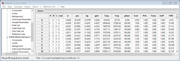
I’ve widened the window so you can see all the columns that are given. With the values of the structure factors and their phases we can now construct density maps for both neutrons and x-rays.

1. Select Phases/PbSO4 from the GSAS-II data tree. In the Fourier map controls section near the bottom, select Fobs for the Map type.

2. Select PWDR PBSO4.CWN: BANK1 for the Reflection set.

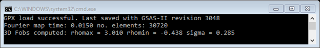
3. Select Compute/Fourier map from the General menu. A map will immediately be calculated via fast Fourier transform techniques. If the project is saved, this map will be included in the project file. The console gives a few lines of output:

and the plot shows the structure (4 atoms) and a green dot which is the highest density point in the map. NB: it might be hidden underneath at atom.

4. Select Draw Options in the Phase data for PbSO4 window. Note the additional controls that have appeared

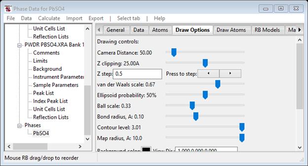
You can lower the contour level and then rotate the drawing around (hold down left mouse button or the mouse wheel) to see the neutron scattering density. It helps to reduce the van der Waals scale to see the density underneath the atoms. You can also slide the structure (hold down right mouse button) to put it where the density is drawn and turning the mouse wheel controls the camera distance (e.g. zoom).

Notice that the density (size of point – really a small octahedron) is higher at the Pb atom & lowest for the S atom; these are in proportion to their neutron scattering lengths.

5. Now let’s try the same thing for the x-ray data. Select the General tab in Phase data for PbSO4 window. Choose PWDR PBSO4.XRA: BANK1 for the Reflection set. Then select Compute/Fourier map from the General menu. A map will be immediately calculated; this will replace the neutron map with the newly made x-ray map. If the project is saved then this map will be in the project. The plot will be redrawn showing the atoms and a small green dot.

6. Again select Draw Options tab, adjust the Contour level and move the drawing around to your liking.

This time only the Pb atoms can be seen in the density map, the S atoms are barely visible at the lower contour level setting and the O atoms are almost invisible. This is also expected based on the relative x-ray scattering power of these atoms; Pb with 82 e^- far outscatters S (16 e^-) and O (8 e^-).